Feature Matching & Stereo Vision
Computer vision project exploring feature detection, stereo correspondence, and depth estimation using OpenCV.
Feature Detection and Mapping
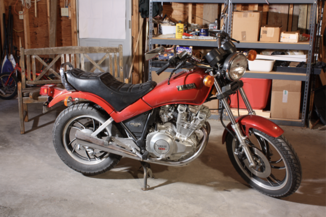
The first step in any stereo vision pipeline is identifying unique, repeatable points in an image areas that can be reliably recognised from another viewpoint. These are known as keypoints. In this project, a sample motorbike image was used to illustrate how features are extracted before any matching occurs.
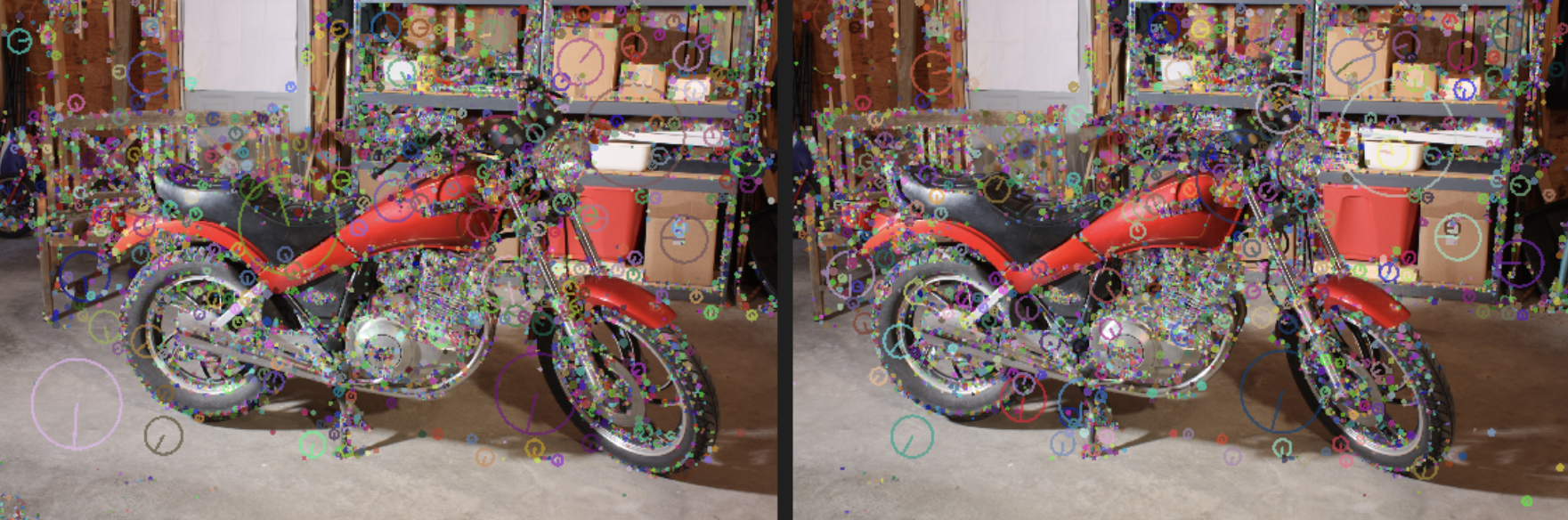
SIFT Feature Detection
The Scale Invariant Feature Transform (SIFT) algorithm was developed by David Lowe (ICCV, 1999).
It identifies keypoints that remain consistent despite changes in scale, rotation, and lighting.
SIFT generates a 128-dimensional descriptor for each keypoint, capturing local gradient patterns that make the feature distinctive and robust.
For the example dataset, approximately 11,761 keypoints were detected in the first image and 11,928 in the second, each represented as a 128-element feature vector.
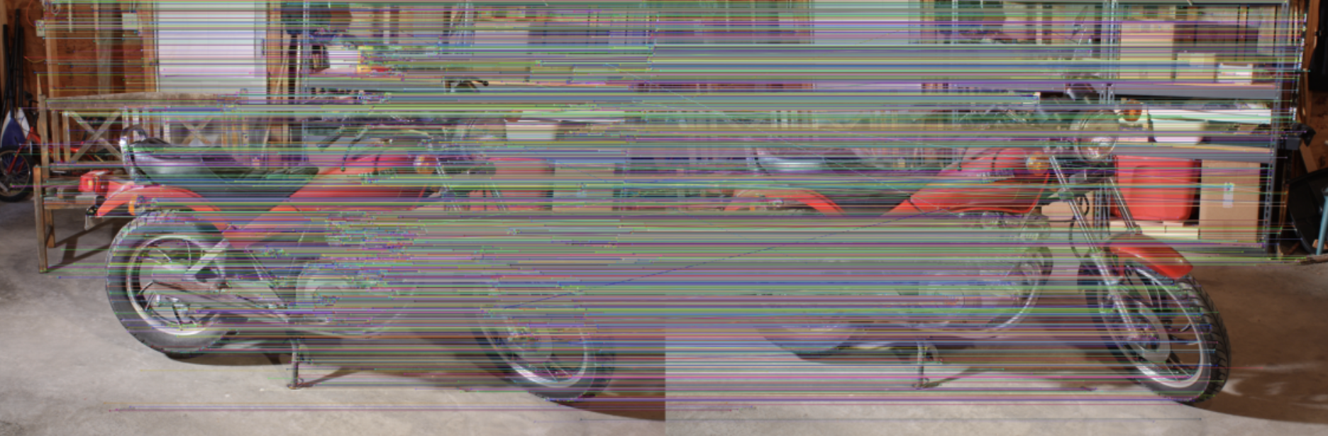
Good Matches
With features extracted from both images, the next step involves matching corresponding points between them. This is typically done using a feature matcher such as the FLANN or Brute-Force matcher in OpenCV. Each match links one keypoint in the left image to a similar descriptor in the right image.
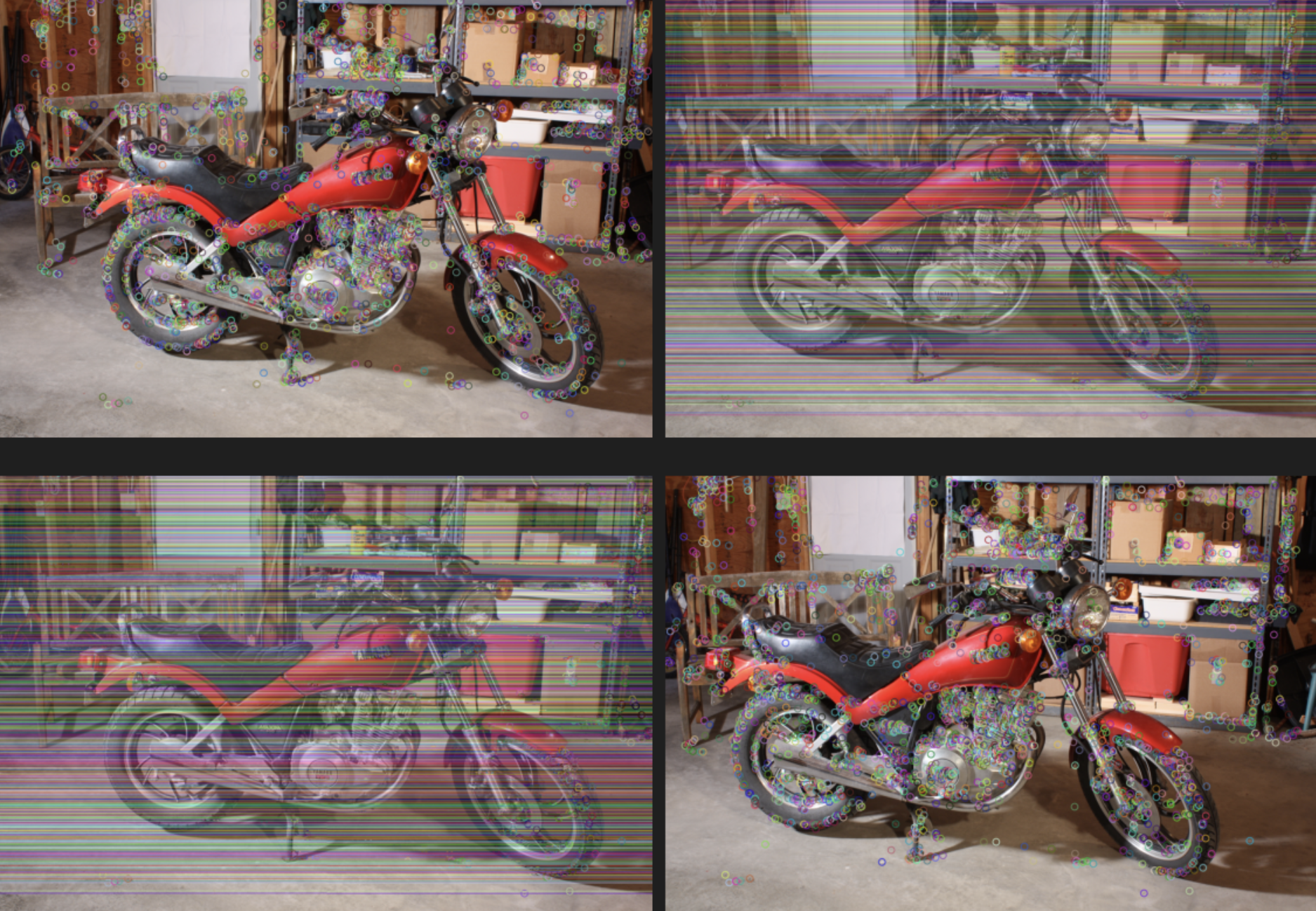
Epipolar Lines
Once good matches are identified, the geometry of the camera setup can be understood through the epipolar constraint.
This ensures that a point in one image must lie along a specific line (the epipolar line) in the other image.
By estimating the fundamental matrix, these lines can be drawn to visualise the spatial relationships between views.
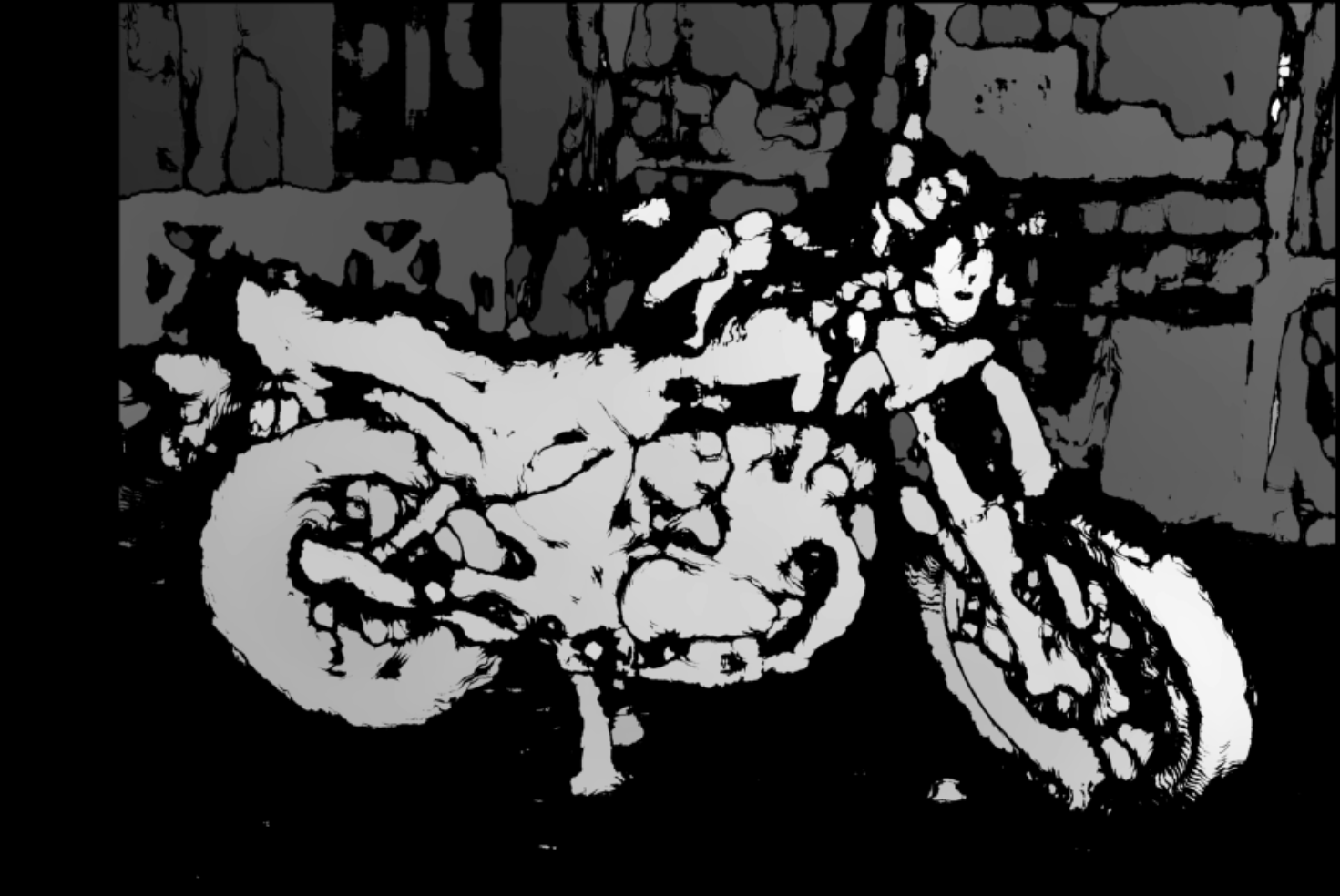
Disparity and Depth Map
The disparity map measures how far apart corresponding pixels are between the left and right images.
Areas with greater disparity are closer to the camera.
OpenCV provides a StereoBM or StereoSGBM algorithm to compute this map,
producing a grayscale output where brighter regions represent closer objects.
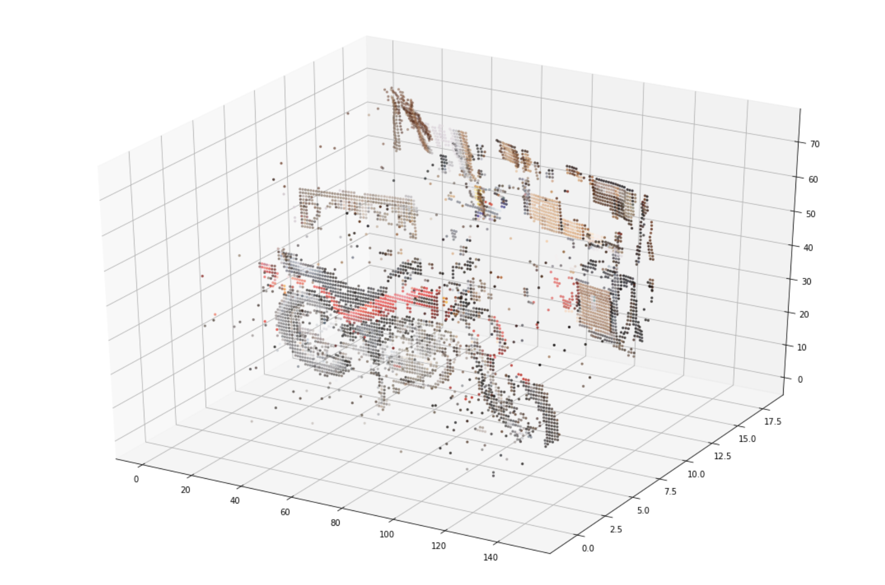
Visualising Depth in 2.5D
The final stage involves projecting the disparity map into a 2.5D depth plot.
This offers a kind-of-3D view of the scene, where depth is inferred from pixel displacement rather than an actual 3D model.
It gives a clear representation of how the stereo pipeline captures geometric structure.
Summary
This project gave me insight into how stereo vision works from detecting features, matching points and more. It showed me the importance of robust descriptors like SIFT for maintaining consistency across viewpoints and demonstrated how geometric reasoning (through epipolar lines and disparity) enables machines to perceive depth.